Table of contents
Notes for figuring out how to read/write those R formulas used in
lmerandbrms.
Summary
I needed to understand a Bayesian mixed-effect model and write about it. It was time to figure out how those R formulas work.
The evolution of those formulas (Under construction)
- Wilkinson-Rogers syntax. The original? most basic? kind of formula. As seen in
lm(y ~ x + z).
Wilkinson-Rogers-Pinheiro-Bates https://twitter.com/BatesDmbates/status/1111283948615802881
throw Burkner on the end there for the brms extensions to it
brms accepts formulas in the form response | aterms ~ pterms + (gterms | group).
Formula components
aterms: specialbrmssyntax, like usingtrial(5)to sneak in the value of \(n=5\) in \(Binomial(n, p)\).pterms: population-level terms.gterms: group-level terms.group: grouping factor.1: intercept, often omitted when there’s another predictor. So(1+x|g)is the same as(x|g).
TODO: confusing frequentist language below:
Group-level terms
There can be multiple group-level effects gterms and multiple grouping factors group.
(1 | random): random group intercepts only(0 + fixed | random) = (-1 + fixed | random): random slopes only(0 + fixed | random) + (1 | random): random slopes and intercepts, independent. Alternatively:(fixed || random).(1 + fixed | random) = (fixed | random): correlated random slopes and intercepts, see below for the correlation coefficients.(1 + gterms |<ID>| group): according tobrmsdocumentation, if there are multiple group-level termsgtermsfor the same factorgroup, we can choose to model the correlations among thosegterms. This is possible for when those group-level terms are in different forumlas, say in a non-linear model.|<ID>|tags the grouping factor and allgtermswith the same ID will be modeled as correlated.- Example: if the model says
(1+x|2|g)and(1+z|2|g),brmswill estimate the correlation between the group-level effects ofxandz.
- Example: if the model says
Incremental examples
Note:
sstands for subject/grouping parameter
1+(1|s)
- Not a mixed-effects model
- Estimates two parameters, \(\beta_0\) and \(\beta_1\)
- \(Y_{si} = \beta_0 + \beta_1 X_i + e_{si}\)
x+(1|s)
- Random intercepts, fixed slopes
- Estimates three parameters:
- A global intercept, \(\beta_0\)
- A global estimate for the fixed effect (slope) of
x, \(\beta_1\) - How much the intercepts for levels in
sdeviate from the global intercept, \(\sigma_{00}\).
- \(Y_{si} = (\beta_0 + S_{0s}) + \beta_1 X_i + e_{si}\)
- \(S_{0s} \sim \mathcal{N}(0, \sigma_{00}^2)\)
x+(0+x|s)+(1|s)
- Independent random slopes and intercepts
- Estmiates four paramters:
- How much the slopes for levels in
sdeviate from the global slope \(\beta_1\), \(\sigma_{11}\). Or how much the effect ofxwithin each level ofsdeviates from the global effect ofx.
- How much the slopes for levels in
- Note that \(S_{0s}\) and \(S_{1s}\) are drawn from two independent distributions with different variances.
- \(Y_{si} = (\beta_0 + S_{0s}) + (\beta_1 + S_{1s}) X_i + e_{si}\)
- \(S_{0s} \sim \mathcal{N}(0, \sigma_{00}^2)\)
- \(S_{1s} \sim \mathcal{N}(0, \sigma_{11}^2)\)
x+(1+x|s)
- Correlated random slopes and intercepts
- Estmiates five paramters:
- Correlation between intercepts \(S_{0s}\) and slopes \(S_{1s}\), \(\sigma_{01}\).
- \(Y_{si} = (\beta_0 + S_{0s}) + (\beta_1 + S_{1s}) X_i + e_{si}\). Same as above, but
- \(\begin{pmatrix}S_{0s} \\ S_{1s}\end{pmatrix} \sim \mathcal{N}\left( \begin{pmatrix} 0 \\ 0 \end{pmatrix},\begin{pmatrix} \sigma_{00}^2 & \sigma_{01}\\ \sigma_{01} & \sigma_{11}^2 \end{pmatrix}\right)\)
Understanding x+(1+x|ID|g)
library(stats)
library(rstan)
library(brms)
library(tidyverse)
library(knitr)
library(kableExtra)
rstan_options(auto_write = TRUE)
options(mc.cores = parallel::detectCores())
The basic distributional model
We can start with a simple distributional model with a normally distributed response variable. The mean \(\mu\) is estimated with the formula x + (x |group). The variance parameter \(\sigma\) is assumed to be the same across observations. The brms model output summarizes which parameters get estimated:
# m <- brm(
#   brmsformula(y ~ x + (x |group), family = gaussian()),
#   data = df,  control = list(adapt_delta = .99),
#   prior = priors1)
m1
## Family: gaussian
## Links: mu = identity; sigma = identity
## Formula: y ~ x + (x | group)
## Data: df (Number of observations: 30)
## Samples: 4 chains, each with iter = 2000; warmup = 1000; thin = 1;
## total post-warmup samples = 4000
##
## Group-Level Effects:
## ~group (Number of levels: 3)
## Estimate Est.Error l-95% CI u-95% CI Rhat Bulk_ESS Tail_ESS
## sd(Intercept) 0.12 0.27 0.00 0.70 1.00 617 549
## sd(x) 0.09 0.15 0.00 0.55 1.01 640 503
## cor(Intercept,x) -0.04 0.62 -0.97 0.96 1.00 1806 1590
##
## Population-Level Effects:
## Estimate Est.Error l-95% CI u-95% CI Rhat Bulk_ESS Tail_ESS
## Intercept 0.02 0.10 -0.16 0.28 1.00 823 449
## x 1.01 0.08 0.87 1.18 1.01 626 330
##
## Family Specific Parameters:
## Estimate Est.Error l-95% CI u-95% CI Rhat Bulk_ESS Tail_ESS
## sigma 0.12 0.02 0.09 0.16 1.00 2010 1284
##
## Samples were drawn using sampling(NUTS). For each parameter, Bulk_ESS
## and Tail_ESS are effective sample size measures, and Rhat is the potential
## scale reduction factor on split chains (at convergence, Rhat = 1).There are five parameters for the group-level and population-level combined, as we have seen above. The sixth paramter is the \(\sigma\) for the normal distribution.
With a submodel for variance
Sometimes we are interested in the variance \(\sigma\) across groups. We add a submodel for \(\sigma\), x + (x|group), just like the one for \(\mu\) (the Family Specific Parameters in m1).
Independent group-level covariances
# f2 <- brmsformula(
#   y ~ x + (x|group),
#   sigma ~ x + (x|group),
#   family = gaussian())
# ...
m2
## Family: gaussian
## Links: mu = identity; sigma = log
## Formula: y ~ x + (x | group)
## sigma ~ x + (x | group)
## Data: df (Number of observations: 30)
## Samples: 1 chains, each with iter = 2000; warmup = 1000; thin = 1;
## total post-warmup samples = 1000
##
## Group-Level Effects:
## ~group (Number of levels: 3)
## Estimate Est.Error l-95% CI u-95% CI Rhat Bulk_ESS Tail_ESS
## sd(Intercept) 0.07 0.12 0.00 0.44 1.01 384 541
## sd(x) 0.08 0.14 0.00 0.50 1.00 261 204
## sd(sigma_Intercept) 1.24 1.74 0.05 6.38 1.00 250 245
## sd(sigma_x) 1.04 1.51 0.02 5.85 1.02 177 188
## cor(Intercept,x) -0.02 0.61 -0.97 0.97 1.00 729 463
## cor(sigma_Intercept,sigma_x) -0.02 0.60 -0.96 0.97 1.01 524 505
##
## Population-Level Effects:
## Estimate Est.Error l-95% CI u-95% CI Rhat Bulk_ESS Tail_ESS
## Intercept 0.01 0.07 -0.14 0.15 1.00 574 546
## sigma_Intercept -2.46 1.16 -4.45 -0.22 1.00 373 303
## x 1.02 0.09 0.90 1.22 1.01 398 286
## sigma_x 0.26 1.12 -2.33 2.61 1.01 123 92
##
## Samples were drawn using sampling(NUTS). For each parameter, Bulk_ESS
## and Tail_ESS are effective sample size measures, and Rhat is the potential
## scale reduction factor on split chains (at convergence, Rhat = 1).Note that there are two correlation terms cor(Intercept,x) and cor(sigma_Intercept,sigma_x).
Resources
- Set up a model formula for use in brms
- Estimating Distributional Models with brms
- lmer cheat sheet | stackoverflow
- R-Sessions 16: Multilevel Model Specification (lme4)
- Using R and lme/lmer to fit different two- and three-level longitudinal models - R Psychologist
- GLMM FAQ
- Fitting linear mixed-effects models using lme4
- Barr, Dale J, R. Levy, C. Scheepers und H. J. Tily (2013). Random effects structure for confirmatory hypothesis testing: Keep it maximal. Journal of Memory and Language, 68:255– 278.
](/images/lme4.png)
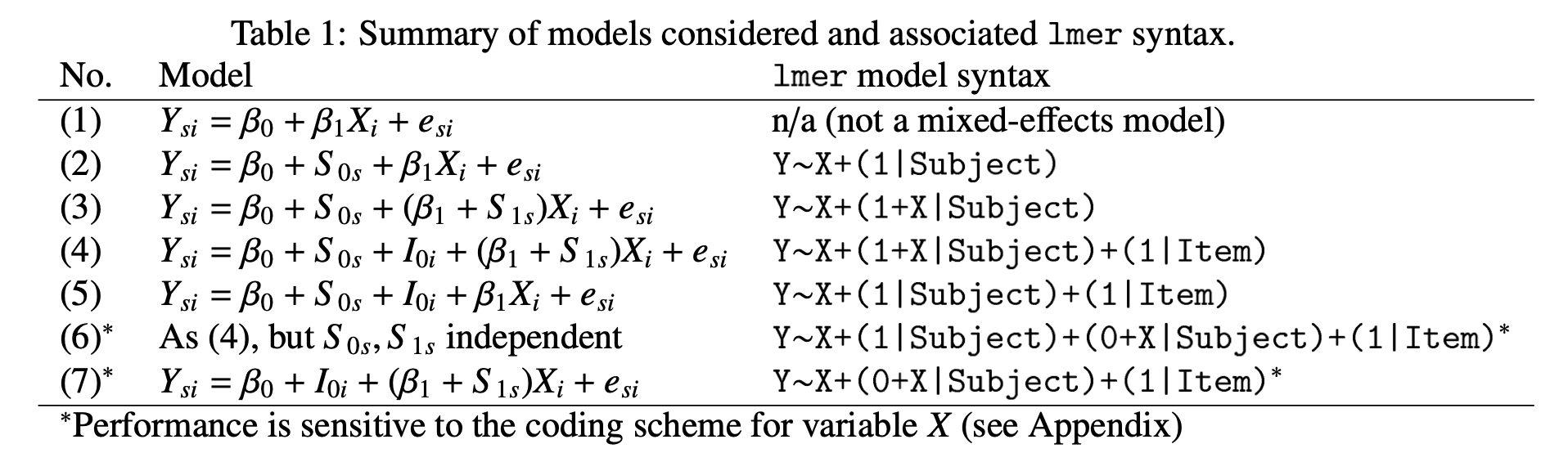
Figure 2: Barr et al. 2013